In an era where AI dominates headlines and transforms industries, there’s never been a better time to understand the fundamental concepts that power these technologies. This series aims to demystify deep learning for software engineers and tech professionals who want to contribute to this revolutionary field without getting lost in mathematical complexity.

This series distills essential deep learning concepts, ideal for software engineers seeking skill expansion without a PhD or full-time research, as I transitioned from a typical engineer in B2B & SaaS. (If you’re interested about my background. feel free to checkout https://www.vithu.site/).

I’m starting this series because I believe the current AI revolution will attract many talented individuals who want to make meaningful contributions. While there are excellent in-depth resources available (and I must give credit to Andrej Karpathy’s exceptional “Neural Networks: Zero to Hero” YouTube series which inspired much of this content), It may be a long on-going series. For now, I am committing myself to publish at least one article per week on this. sometimes we need a concise summary to get started.

Let’s start with some mathematical aspects that you need to be grounded to become an expert in AI. A good amount of understanding of gradients, derivatives, limits, vectors and few other mathematical components will make your life easier in the upcoming articles.

The notebook for the code used in this article can be found here.

Why Gradients Matter in Deep Learning

At the heart of modern neural networks lies a deceptively simple concept: gradients. These mathematical tools allow neural networks to learn from data by making incremental improvements. Understanding gradients is your first step toward mastering deep learning.

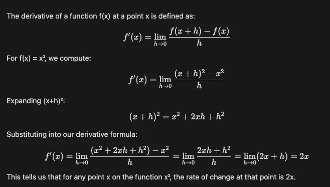
Understanding Derivatives Through Example x², the rate of change at that point is 2x.

Let’s explore why the derivative of x² is 2x. The derivative represents the rate of change of a function, and we can derive this step-by-step.

Building Grad Visualization & Understanding Backpropagation

To truly understand how neural networks learn, let’s build a simple visualization. This will help us visualize how gradients flow through a network.

class Value:
  def __init__(self, data, _children=(), _op=(), label = ''):
    self.data = data
    self.prev = set(_children)
    self.grad = 0.0
    self._op = _op
    self.label = label
def repr(self):
return f"Value(data={self.data})"
def add(self, other):
other = other if isinstance(other, Value) else Value(other)
return Value(self.data + other.data, (self, other), '+')
def mul(self, other):
other = other if isinstance(other, Value) else Value(other)
return Value(self.data * other.data, (self, other), 'x')
def sub(self, other):
other = other if isinstance(other, Value) else Value(other)
return Value(self.data - other.data, (self, other), '-')
def truediv(self, other):
other = other if isinstance(other, Value) else Value(other)
return Value(self.data / other.data, (self, other), '/')

This simple class allows us to track computations and their gradients. Let’s use it to create a small computational graph:

An example usage of this value class would be:

a = Value(2.0, label='a')
b = Value(-3.0, label='b')
c = Value(10.0, label='c')
e = a*b; e.label = 'e'
d = e + c; d.label = 'd'
f = Value(-2.0, label='f')
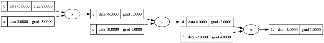
L = d * f; L.label = 'L'

This creates a computation where:

• e = a b = 2 (-3) = -6

• d = e + c = -6 + 10 = 4

• L = d f = 4 (-2) = -8

To visualize this better you can use graphviz as below:

import numpy as np
import matplotlib.pyplot as plt
%matplotlib inline
from graphviz import Digraph

def trace (root):
nodes, edges = set(), set()
def build(v):
if v not in nodes:
nodes.add(v)
for child in v.prev:
edges.add((child, v))
build(child)
build(root)
return nodes, edges
def draw_dot(root):
dot = Digraph(format='svg', graph_attr={'rankdir': 'LR'}) # LR = left to right
nodes, edges = trace(root)
for n in nodes:
uid = str(id(n))
# for any value in the graph
dot.node(name = uid, label = "{ %s | data %.4f | grad %.4f }" % (n.label, n.data, n.grad), shape='record')
if n._op:
# if this value is a result of some operation
dot.node(name = uid + n._op, label = n._op)
# and connect this node to it
dot.edge(uid + n._op, uid)
for n1, n2 in edges:
# connect n1 to the op node of n2
dot.edge(str(id(n1)), str(id(n2)) + n2._op)
return dot

You can invoke the draw_dot now with a value object to get the visualization

dot = draw_dot(L)
dot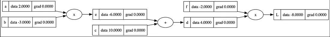

Now comes the magic of neural networks: backpropagation. This is how networks learn by propagating gradients backward through the computation graph.

Let’s breakdown the gradients starting from the node L. we can do this by adding a small difference h to the L directly and utilizing the definition of derivative.

# when direcrly adding a small diff h to L, we can figure out the derivative of L with respect to L by identifying the limit
h = 0.00000001

a = Value(2.0, label='a')
b = Value(-3.0, label='b')
c = Value(10.0, label='c')
e = a*b; e.label = 'e'
d = e + c; d.label = 'd'
f = Value(-2.0, label='f')
L = d * f; L.label = 'L'

L1 = L
L2 = L1 + h
(L2 - L1) / h # This is going to be the derivative of L with respect to L which is 1

Now we can set the gradient of L to be 1.

L.grad = 1

Now let’s calculate the derivative of L with respect to f,

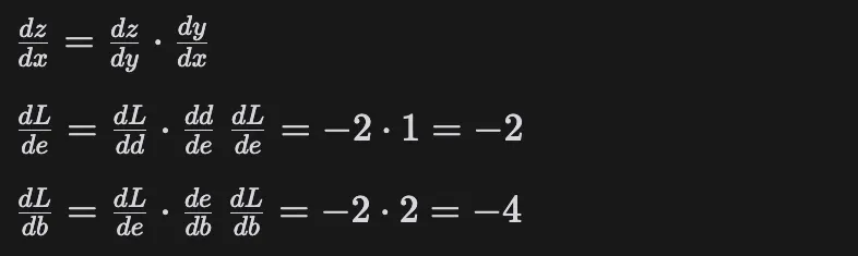
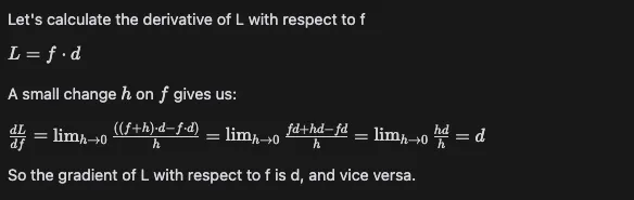Similarly, we can calculate other gradients using the chain rule:

dL/de = dL/dd · dd/de = -2 · 1 = -2

dL/db = dL/de · de/db = -2 · 2 = -4

We can verify this by changing b by a small amount and seeing how L changes:

h = 1

Original computation
a = Value(2.0, label='a')
b = Value(-3.0, label='b')
c = Value(10.0, label='c')
e = a*b; e.label = 'e'
d = e + c; d.label = 'd'
f = Value(-2.0, label='f')
L = d * f; L.label = 'L'
L1 = L  # L1 = -8.0
Computation with b changed by h
a = Value(2.0, label='a')
b = Value(-3.0 + h, label='b')  # b = -2.0
c = Value(10.0, label='c')
e = a*b; e.label = 'e'
d = e + c; d.label = 'd'
f = Value(-2.0, label='f')
L = d * f; L.label = 'L'
L2 = L  # L2 = -12.0
Change in L divided by change in b
(L2.data - L1.data) / h  # = -4.0

Likewise, let’s calculate the derivative of d with respect to e:

Will update the derivative accordingly.

e.grad = 1
c.grad = 1
b.grad = 2
a.grad = -3

Once we update the grad, when we visualize the graph again, we will get the below picture.

Now we’ll use the chain rule to understand the impact of the very first inputs on the end results.

What this means is if we nudge b by 1, the result will change by -4.

This is exactly how a neural network leverages each and every data point to determine the possible outcome at the very end. propagating these gradient backwards from the last output to very first set of inputs is called “backpropagation”. This is the key algorithm used behind almost all the powerful AI models as of today.

Why This Matters

This gradient calculation is the foundation of how neural networks learn. During training:

• The network makes a prediction

• We calculate how wrong the prediction is (the loss)

• We compute gradients to determine how each parameter contributed to the error

• We adjust parameters in the direction that reduces the error

By repeating this process millions of times with different examples, neural networks gradually improve their predictions.

What’s Next?

In the next article, we’ll expand our gradient visualization to handle math operations and see how we can use demonstrate a simple backpropagation. We’ll also explore how these concepts scale to the massive networks powering today’s AI systems.

Understanding these fundamentals will give you a solid foundation to build upon, whether you’re implementing neural networks from scratch or using high-level frameworks like PyTorch or TensorFlow or even directly building AI agents ontop of the foundation models.

Stay tuned for more in this Deep Learning Series, where we’ll continue to demystify the concepts that power modern AI.